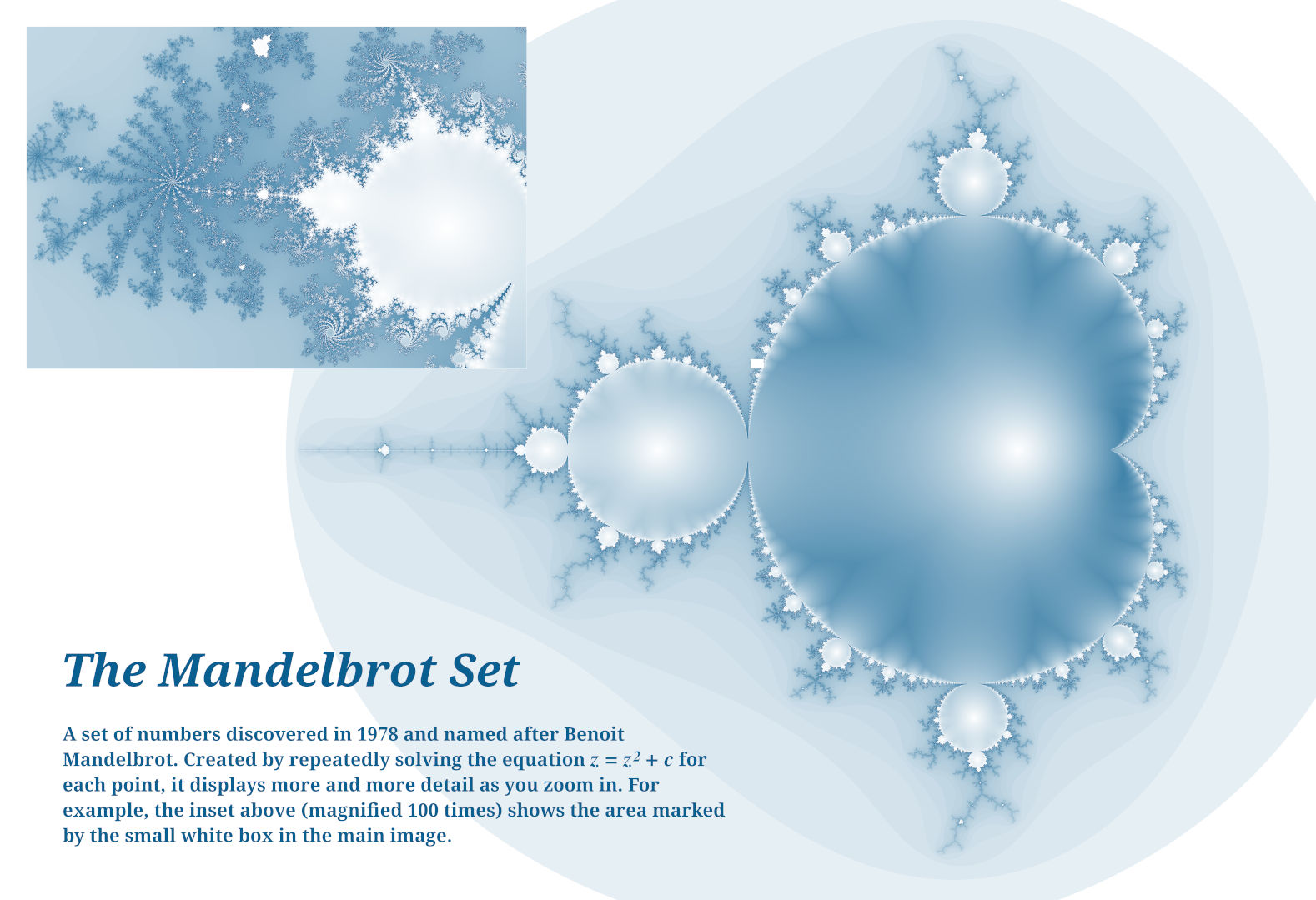
This is a poster created using this method and GIMP to add the text. a full-size 13x19 in at 300 ppi image is available on Google Drive. | Source Code
Using Python, creating images of the mandelbrot set is surprisingly simple.
The Mandelbrot set is one of the most famous fractals in history. With its incredible complexity and intriguing mathematical properties, it is no wonder so many images of it have been created. A quick YouTube search will yield many videos filled with nothing other than minutes of zooming into its infinitely complex border.
However, one of the strangest properties of the Mandelbrot set is the simple function that creates it. Just a few lines of code are required to display its shape. In Python, it is even easier, due to the support of complex numbers.
The Mandelbrot set is defined as the group of numbers on the complex plane which do not diverge after putting them through the function f(z) = z2 + c. The 'complex plane' is a way of visualizing complex numbers, a combination of normal numbers and imaginary numbers (i, or the sqare root of -1).
For example, if you take the number line and add a vertical axis, the new axis represents complex numbers. Anything on that axis is a multiple of i, and anything in one of the quadrants is the sum of a normal and imaginary number (e.g., 1 + 3i).
By looping through points in a grid around the origin and testing each one to see if it grows larger, a simple image of the mandelbrot set can be created.
To execute this in code we first loop through the points. In this case I assume it will be an image, so I use integer values that represent the coordinates of each pixel.
data = []
for y in range(height):
for x in range(width):
Then the x and y values need to be mapped to around the origin. In the code,
zoom will determine how much area is shown. A value of about 0.5
shows the entire set nicely.
a = (x / width - 0.5) / zoom  # map x and y to
b = (y / height - 0.5) / zoom # center and scale
a /= height / width # fix the aspect ratio
Then, convert the coordinates to complex numbers and run the equation. The technical definition is f(z) = z2 + c starting with z = 0 and c as the complex coordinate. Since 02 + c = c, we can just immediately assign c to z in the code.
c = complex(a, b) # covert to complex for computation
z = c # z should start at 0, but will always become c next

color = (0,0,0) # default to inside the set (set the color to black)

for i in range(max_steps):
z = z * z + c

# here abs(z) is used to convert the complex number into a
# comparable value. This lets us check to see if it is growing
# too large to be a part of the set

if (abs(z) > escape_radius): # the number diverges
    color = (255,255,255) # assign the background color (white)
    break # stop the loop; we're done

data.append(color)
Above, max_steps is the number of times the function is repeated
before assuming the number is in the set. The higher the number of steps, the
more detail that is visible, but it takes more time. Similarly, escape_radius
is the limit beyond which we assume the number is outside the set. (2.1 is a good
value) After this, we can simply assign the colors to an image.
from PIL import Image

output = Image.new(
"RGB" # mode (RGB or RGBA usually)
(width, height) # size
)
output.putdata(data)
output.save("mandelbrot.png")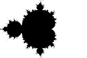
From this sample output, you can already see the incredible detail, but the
the colors are a bit bland. To fix this, we can take a few of the other variables and
use them to add shading. For the outside, the number of steps it takes to get outside
the escape_radius works well.
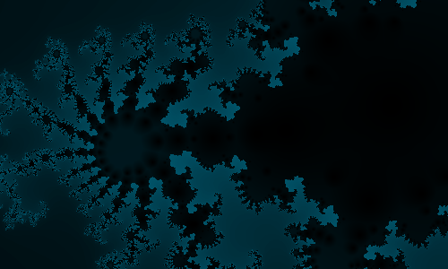
For the inside, I like to use a method called an 'orbit trap.' This keeps
track of how close the point gets to the 'trap' loaction, usually the origin,
and uses the minimum value to shade the figure.
detail_color = (130, 170, 255) # a light blue for now
# the shade values should be between 0 and 1
# so it can be used to multiply with the color
min_orbit = 1.0

for i in range(max_steps):
z = z * z + c
# use abs(z) as the distance to the origin (0,0)
min_orbit = min(abs(z), min_orbit)

if (abs(z) > escape_radius): # the number diverges
    # scale the iteration to [0,1] and assign it to value
    value = i / max_steps
    break

# otherwise:
value = min_orbit

# multiply each color channel by the value to
# make it lighter or darker
color = tuple(
int(value * rgb) for rgb in detail_color
)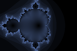
This creates a much more interesting image with more color and detail. As a side
note, it is now clear that the image is off-center. This can be fixed by simply
adding a -= 0.65 to the code to re-center it.
Now that the basic code is done, we can move on to more interesting parts: customizing
the image. A good start would be to request user input for some of the variables such
as height and width. Another quick change would be to add
a coordinates variable and add it to a and b
to customize the center location. This helps if you want to zoom into some of the
infinite finer detail near the borders. A few interesting locations are
(0.001643721971153, 0.822467633298876) for a long zoom into
one of the spirals or (-0.725, 0.24) for a closer look at the
middle.
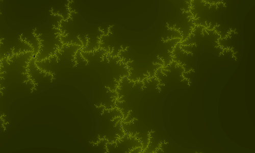
Green: (0.001643721971153, 0.822467633298876) at around 500x zoom.
Blue: (-0.725, 0.24) at 50x zoom
If a solid black background is not enough, you can also modify the colors displayed. Using a custom mix function, you can blend two colors based on the value. Or, you could use Hue Lightness Saturation colors instead of Red Green Blue and use a built-in color library to convert the values back to RGB for the image.
# mixes two colors based on a percentage value
def mix(percent, detailColor=(255,255,255), backColor=(0,0,0)):
outColor = [0,0,0]
for n in range(3):
    d = detailColor[n]
    b = backColor[n]
    outColor[n] = int(d * percent + b * (1 - percent))
return tuple(outColor)
from colorsys import hls_to_rgb
# loop through and convert to RGB
for pixel in imageData:
colors.append(
tuple(
# the function provides values from [0,1], the image should
# be from [0, 255]
int(rgb * 255) for rgb in hls_to_rgb(pixel[0], pixel[1], pixel[2])
)
)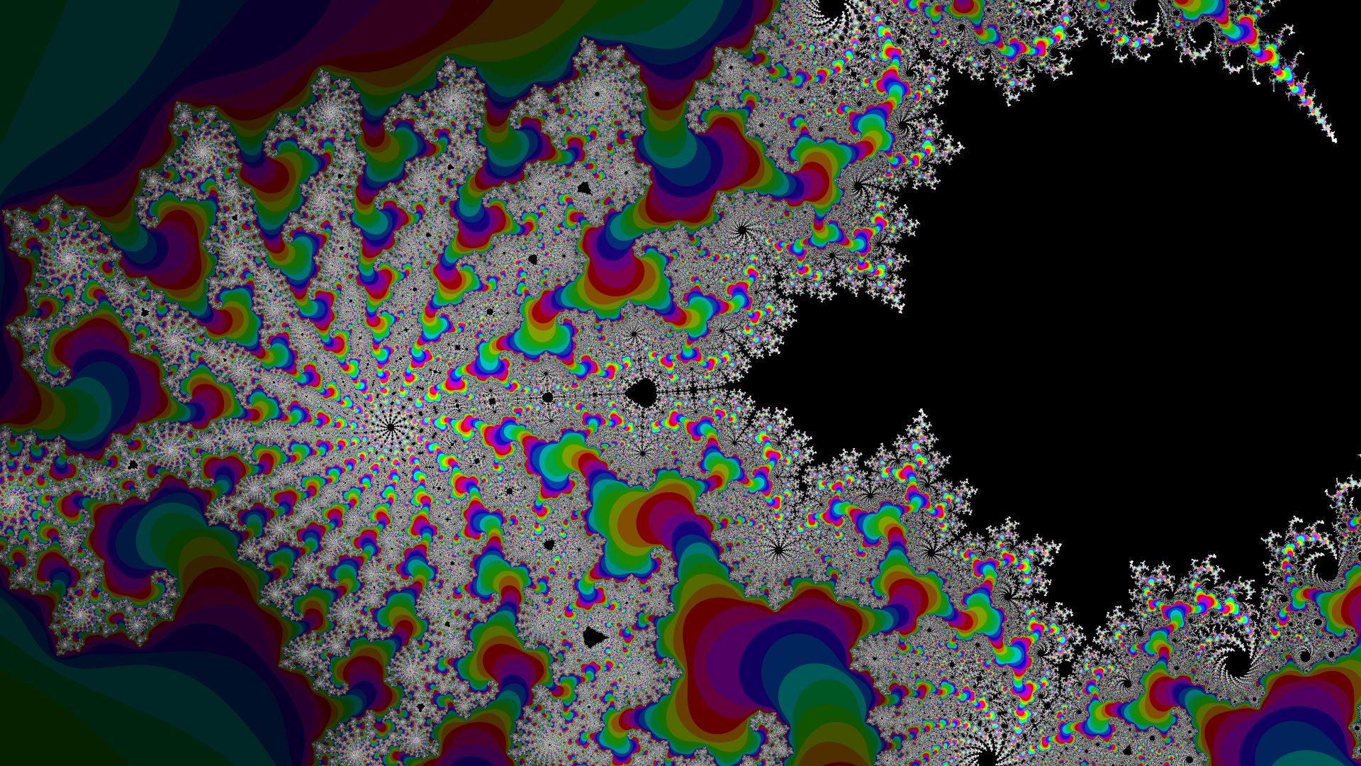
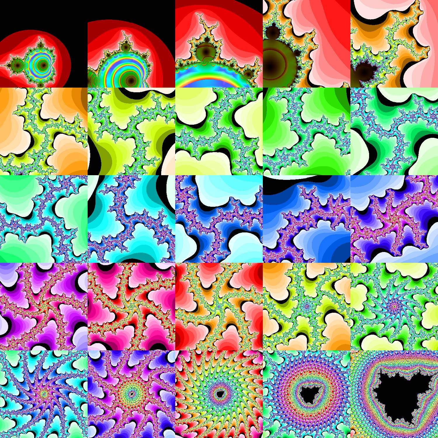
An example of using the step to define the hue. This could have used a few more samples with the antialiasing I describe below, but it already took more time than I wanted with nine.
If you ran any of this code, you may have noticed that it takes quite a bit of time for larger images. This is because of the large number of times each loop has to run. To reduce this time, you could take better advantage of the computer's power through multithreading. This allows the program to run more than one pixel at a time, greatly decreasing the time required to finish. The best way to do this would be to use compute shaders to run each pixel fully parallel on the graphics card (it is made for calculating images after all), but for simplicity I used Python's built-in multiprocessing library.
from multiprocessing import Pool
The Pool object provides a very useful way to calculate large
lists of numbers. Using the .map function, it allows you to run
a single function on a large range of numbers. So, we can use it to generate the
image data like this:
# the Pool will only provide a single value, so
# we need to change it to work as coordinates
def convertForPixel(n):
# get the x coordinate from the remainder of division with the width
x = n % width
# and the y coordinate by floor division
y = n // width
calcPixel(x, y) # calculates the color using the process above

# the number of processes to run simultaneously
# it should be equal to the number of cores on the CPU
# mine has 8 cores, so:
pool = Pool(processes=8)
imageData = pool.map(
convertForPixel, # the function to use
range(width * height) # a list of values to give to the function
)
pool.close()
Using this method, I have managed to increase the speed by nearly three times.
For one final improvement, let's focus on smoothing out the grainy pixels. If you take a look at the image above, you can see that near the edges, where there is a lot of detail, the picture strats to look like a grainy mess. This is because the detail is much smaller than a pixel, so there is not a smooth transition between them. To fix this, we can calculate multiple points, each slightly apart, for every pixel and average them together. This should help get rid of some of the sharp contrasts between pixels, but it is very computationally expensive. For this reason, I did not bother using it for most of my images.
# for each pixel:

def convertForPixel(n):
# get the x coordinate from the remainder of division with the width
x = n % width
# and the y coordinate by floor division
y = n // width
sumc = [0,0,0]
for sx in range(samples):
for sy in range(samples):
# center the samples around (x,y)
newX = x + (sx / samples - 0.5)
newY = y + (sy / samples - 0.5)
sc = calcPixel(newX, newY)
for n in range(3):
  sumc[n] += sc[n]
return tuple(i / samples / samples for i in sumc)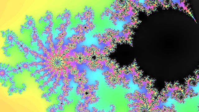

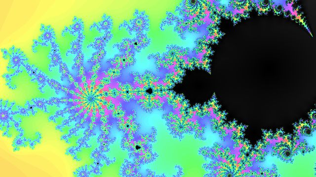
From first to last: No extra samples, four samples (2x2), sixteen samples (4x4). Here you can see the disadvantage to averaging the samples before converting them to RGB. The very dense areas tend to have average values, which means a hue of 0.5. This causes the green tint near the edges.
from colorsys import hls_to_rgb
from multiprocessing import Pool
from PIL import Image

res = 1 # change for a larger/smaller image
width = int(1920 * res)
height = int(1080 * res)
zoom = 0.5
max_steps = 30
escape_radius = 2.1
# detail_color = (130, 170, 255) # unused
coordinates = (-0.65, 0.0)
samples = 2

data = []
def calcPixel(x, y):
a = (x / width - 0.5) / zoom  # map x and y
b = (y / height - 0.5) / zoom # to center
a /= height / width # fix aspect ratio
a += coordinates[0]
b += coordinates[1]
c = complex(a, b) # covert to complex for computation
z = c # z should start at 0, but will always become c next
min_orbit = 1.0
hue = 0.5
value = 1.0
sat = 0.0
for i in range(max_steps):
    z = z * z + c
    # use abs(z) as the distance to the origin (0,0)
    min_orbit = min(abs(z), min_orbit)

    if (abs(z) > escape_radius): # the number diverges
        # scale the values to [0,1]
        value = 0.7
        hue = i / max_steps
        sat = 1.0
        break
    value = min_orbit
color = tuple(
    [hue, value, sat]
)
return color

# the Pool will only provide a single value, so
# we need to change it to work as coordinates
def convertForPixel(n):
# get the x coordinate from the remainder of division with the width
x = n % width
# and the y coordinate by floor division
y = n // width
sumc = [0,0,0]
for sx in range(samples):
for sy in range(samples):
  # center the samples around (x,y)
  newX = x + (sx / samples - 0.5)
  newY = y + (sy / samples - 0.5)
  sc = calcPixel(newX, newY)
  for n in range(3):
    sumc[n] += sc[n]
return tuple(i / samples / samples for i in sumc)

# the number of processes to run simultaneously
# it should be equal to the number of cores on the CPU
# mine has 8 cores, so:
pool = Pool(processes=8)
imageData = pool.map(
convertForPixel, # the function to use
range(width * height) # a list of values to give to the function
)
pool.close()

# loop through and convert to RGB
def modifyColor(pixel):
return tuple(
  # the function provides values from [0,1], the image should
  # be from [0, 255]
  int(rgb * 255) for rgb in hls_to_rgb(pixel[0], pixel[1], pixel[2])
)

newPool = Pool(processes=8)
colors = newPool.map(
modifyColor,
imageData
)
newPool.close()

output = Image.new(
"RGB", # mode (RGB or RGBA usually)
(width, height) # size
)
output.putdata(colors)
# output.save("mandelbrot.png")
output.save("mandelbrot.jpeg", progressive=True, quality=80)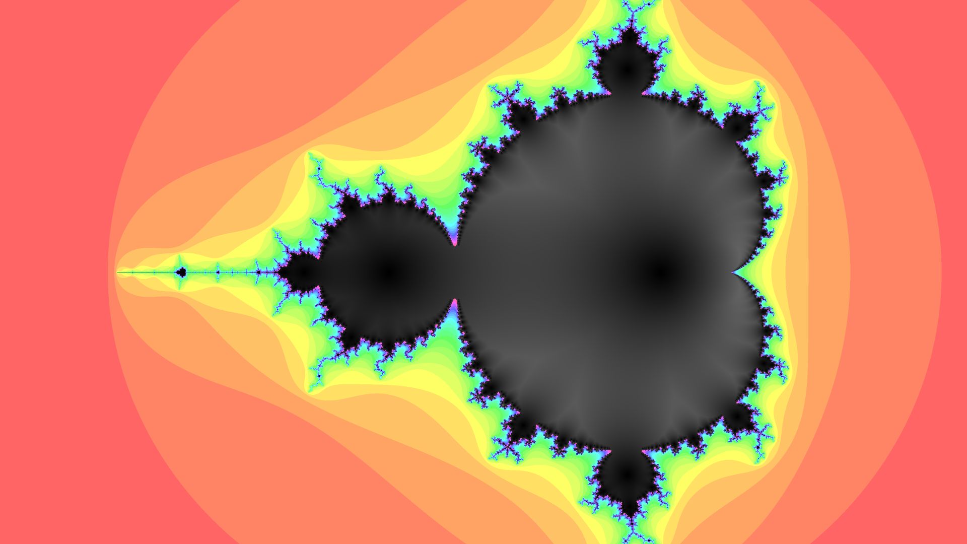
A sample output
As a side note, this code can be easily modified to create
Julia Sets
by assiging a static value to c and setting z to the
complex coordinate. These sets are just as detailed and impressive, and possibly
even more beautiful due to their symmetry.
c = 0.1 + 0.65j # a set I like
z = complex(a, b)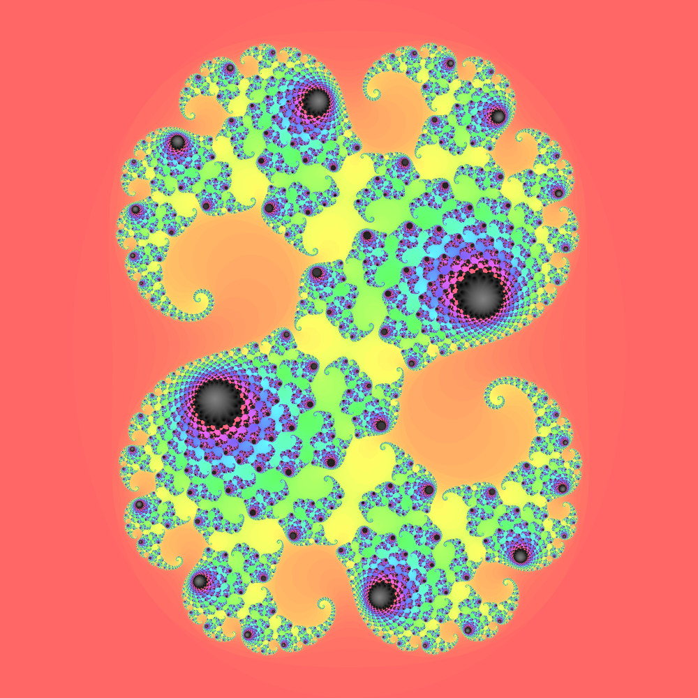
Hopefully, this tutorial has helped you create beautiful images of the Mandelbrot set. If you are interested in learning more, visit the main tutorials page for more resources, or check out my Julia Set Creator. Otherwise, enjoy these images I created using this technique, or view the source code for each.
This is a poster created using this method and GIMP to add the text. a full-size 13x19 in at 300 ppi image is available on Google Drive. | Source Code
A long zoom into (0.001643721971153, 0.822467633298876). A full resolution version of this image is available on Google Drive. | Source Code